Thursday, August 4, 2016
Week Ten
Our poster presentation at the MID-SURE undergraduate research conference was a great experience for improving communication skills to a general audience. The data obtained from the simulations were saved to the schools hard drives. Considering the number of findings we've obtained from the simulation, we plan to work on a paper for the rest of the summer to submit to the 2nd Thermal and Fluids Engineering Conference: https://www.astfe.org/tfec2017/.
Week Nine
We spent a majority of this week working on a poster of our research to present to the MID SURE undergraduate research conference at Michigan State University. Due to the fact that we have a large number of findings from our oil jet study, we decided to only display the results of the impingement areas and the hydraulic dive, as well as visual images of the evolution of the jet over time. The poster was reviewed and accepted by our adviser, Dr. Guessous.


Friday, July 15, 2016
Week Eight
With our time at Oakland University starting to wind down, Morgan and I spent a great deal of time this week organizing data in order to implement it in our paper and poster presentation. Along with this work we attended an interesting lecture on internal combustion engines given by Dr. Zhao, a new professor at Oakland University who graduated from Princeton. Additionally, we attended a poster presentation workshop given by Dr. Dean, where he covered the Do's and Don'ts and other guidelines for giving an effective poster research presentation. This workshop came at a great time, as the MID-SURE Undergraduate Research Conference is being held at Michigan State University on July 27, less than 2 weeks away!
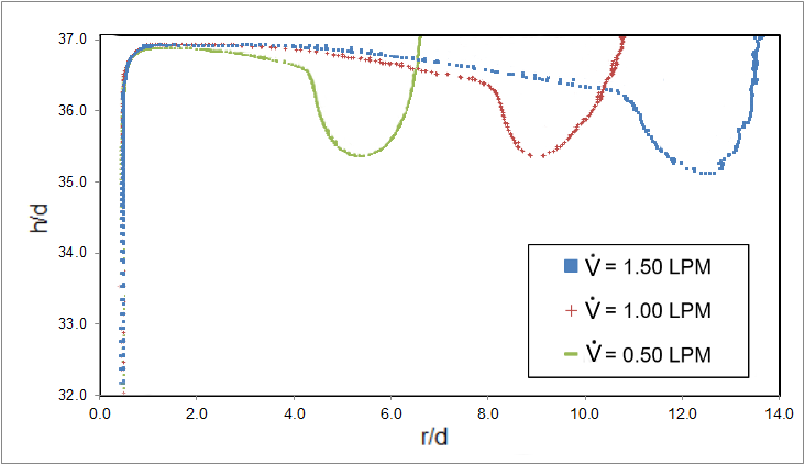

With all that being said, there was still plenty of research going on in our little Dodge Hall enclave. We generated some good plots that illustrates and compares the hydraulic jumps of our three cases. Below is some delicious eye candy, courtesy of Morgan Jones.
Here we are looking at the edge of the impingement area in a region between two streams. This bubble-like formation is a hydraulic jump. Also, notice how the distance progressively gets larger and larger away from the origin. This is just showing that given a higher flow rate, the impingement area is bigger.
Intermission time. Whilst perusing the Internets for a CFD question we were interested in, I found a thread on a CFD help forum with a few CFD-related jokes, if you could imagine there would be such a thing! A few sardonic individuals came up with some quippy mnemonics for CFD that I thought I would share with you:
CFD - Colorful Figure Delivery
CFD - Colors for Directors
CFD - Cleverly Forged Data
You can't deny that there isn't at least a small bit of truth to these...
Back to business! As we defined at the beginning of the summer research, one of the most important things we wanted to look at was the impingement area for the three cases. That is, given a certain flow rate, how big is the impingement area going to be and how much is that going to cool down the piston? Below is a graph comparing the impingement areas for our three cases:
Quantitatively speaking, the 1.0 LPM case's impingement area is 57% larger than the 0.5 LPM case. Furthermore, the 1.5 LPM case area is 69.8% and 166.5% larger than the 1.0 and 0.5 LPM cases, respectively. In short, if you squirt more oil at the bottom of the bottom of the piston, the more the piston will get cooled down. However, it's not that simple as there are other important parameters to look at; such as possible oil misting and parasitic engines losses from the oil pump. Further research is being done (though not currently by us) on how much oil is ideal for cooling down pistons.
Well, folks, that's it for this week. Be sure to come back next week for more exciting CFD news from Dodge Hall!
Friday, July 8, 2016
Week Seven
After a relaxing 4th of July weekend, Morgan and I were back in the lab doing data analysis and working on the American Society of Thermal and Fluids Engineers (ASTFE) paper. Although the paper isn't due until September, we've been chipping away at it to make things considerably easier in the future. The big motivation behind writing this paper is to get it published and to attend the ASTFE conference in Las Vegas next April where we'll present our project.
As the weeks go by, we've been making steady progress with both the paper and the data analysis. After some grid-mesh adaptions we made last week the simulations powered through the weekend to yield some interesting results for us this week. For the 11 m/s case, we refined the grid near a section where two streams were merging together. After letting that case run for a few more days, we found that the streams had separated. Whether that's due to our mesh adaption or a yet-to-be-discovered flow pattern, it is not clear.
This week we also calculated the distances between the streams for the three cases, as well as the average distance. It seems that the average distance for all the cases is between 1.32 and 1.37 cm, regardless of how many streams the case may have. In addition, we calculated the impingement area for each case as a function of time, but focusing on the small fluctuations that are observed at near-steady state. We can't say that any given case reaches exactly steady state as there are always slight changes in the area, but for all intents and purposes, these changes are so small that any deviation from the average value is negligible.
As a highlight, this week Morgan found a new way to calculate the jet impingement region thickness. The old way involved manually converting polar coordinates to Cartesian coordinates to generate a given plane. Once that plane was made, lines were created at set distances within those planes with their values plotted in order to get a select few thickness values. These lines and planes were meticulously created between and at stream locations. As thrilling as that sounds, Morgan decided to reinvent the wheel of tedious plane analysis. However, he not only reinvented the wheel, he created a Mercedes Benz Silver Lightning method of finding these thickness values. Behold! Feast your eyes upon the glory of Morgan's Method:
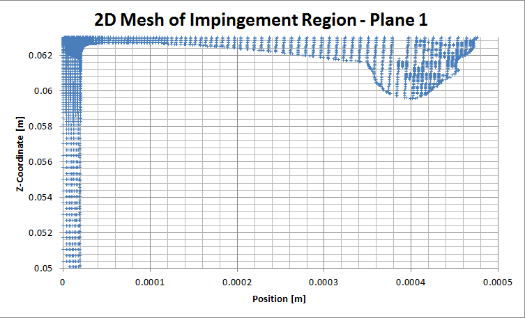 |
| This is so much more than your ordinary, every day Microsoft Excel plot. What you are seeing is a revolutionary way of doing CFD analysis. Simply scroll your mouse over a point, and it will give you a representative thickness value! (Hint: you can't actually scroll over this image to get a value, you'll have to come to our lab to have access to our Top Secret Excel documents.) |
Like any good invention, the highly-coveted secrets behind this method are patented (pending) and are reserved only for the most privileged members of the Oakland's prestigious CFD community...
Friday, July 1, 2016
Week Six
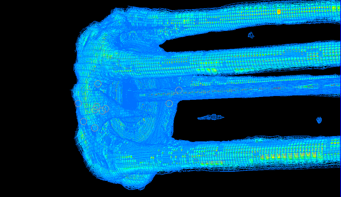
Welcome back! This week there weren't any AERIM events to go to so we had plenty of time to use towards lab work and meeting with Dr. Guessous and Sangeorzan to discuss our results. During these meetings, we found that it was necessary to do a little digging in order to find the best Volume Fraction (VF) cut off range for our data analysis. This volume fraction cut off point is used to show the area of oil on a given plane. If it is too low, as in the picture below, our area will include too much air. If it is too high, one may be neglecting too much oil and thus the mass flow rate is drastically reduced.
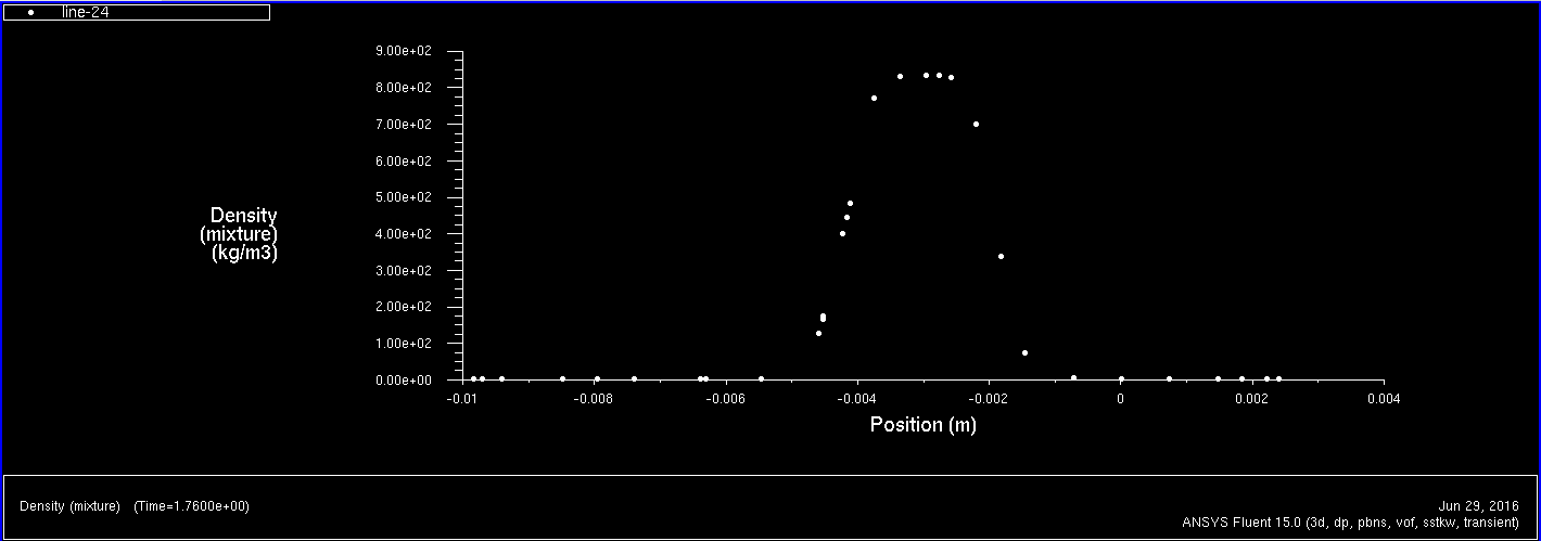
So, in order to effectively consider our VF cut off point, we made plots of density and Volume Fraction at certain distances across the cross-section of a stream. The way Fluent calculates Mass Flow Rate is based off of density. Additionally, there is a direct correlation between density and the volume fraction cut off, as can be seen below.
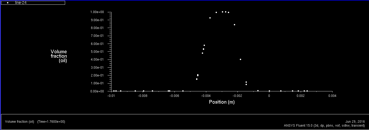
After doing much more analysis concerning the VF cut off point, we decided that a cut off point of 5% would be optimal as it not only clips out the air from calculations, but it also contains the bulk of the oil.
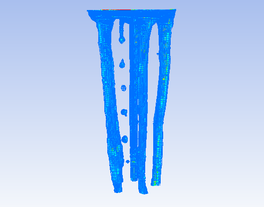
In other news, we're also investigating the formation of a stream on our 3.64m/s case. Below is an image of a drip that is not quite a stream yet. We're refining the mesh here and continuing this simulation to see if indeed a full-fledged stream forms.
 |
| This is an oil Volume fraction from 0 to 1. Notice that this is the area of the entire top plate because it also includes air in its area calculation. |
 |
| This is an impingement area where the Volume Fraction cut off is a 0.05, or 5%. |
 |
After doing much more analysis concerning the VF cut off point, we decided that a cut off point of 5% would be optimal as it not only clips out the air from calculations, but it also contains the bulk of the oil.
In other news, we're also investigating the formation of a stream on our 3.64m/s case. Below is an image of a drip that is not quite a stream yet. We're refining the mesh here and continuing this simulation to see if indeed a full-fledged stream forms.
 |
| A prettier, side angle view that shows the early formation of a stream. |
Thursday, June 23, 2016
Week Five
This week Morgan and I were back at it inside our simulation cave. We achieved some good progress in analyzing the 7.35 and 3.64 m/s cases. Instead of first telling you about it, I'll show you some interesting pictures we generated in CFD-Post and then describe them to you.
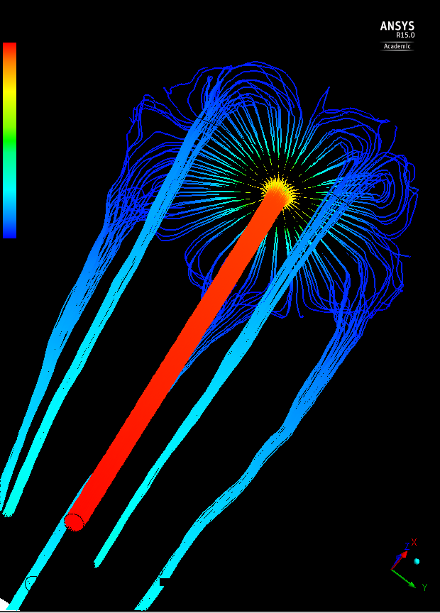
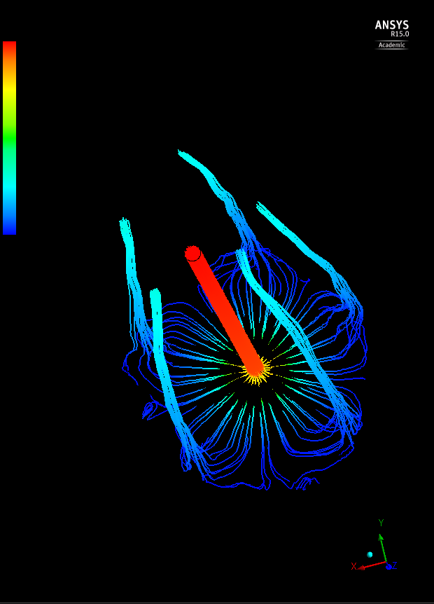
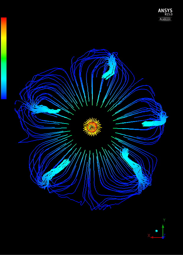
What these cool jellyfish-like pictures are showing are the streamlines of the oil at the impingement area. We can see how and where the downward streams are developing. One thing we would like to do is investigate why they are developing in a given area as well as why they are not equidistant from each other, given an equal surface tension parameter.
Here we have a bottom view where we can see the streamlines forming off of the impingement area. At the very bottom, we have a gathering cluster of streamlines. While most of these will inevitably find their way to the stream to the left and right, we have seen that this is where some drops of oil have fallen. With a slight increase in velocity, we believe this could be where the 6th stream is supposed to develop.
In this picture we have a side view of a section of the impingement area. We can easily estimate the thickness, however, we would like to quantify the thickness of the impingement area as a function of the radial velocity and velocity gradient.
Week Four
This was indeed a very packed and exciting week filled with analysis, meetings, presentations, and vehicle test-driving. Monday and Tuesday were spent doing data analysis on the 7.35 and 3.64 m/s cases. Additionally, we were preparing for our presentation on Wednesday. After said presentation on Wednesday, Morgan and I met with Dr. Guessous and Sangeorzan to discuss the results of our project as well as its future direction. We want to be able to characterize the thickness of the impingement area and relate it to the radial velocity gradient with respect to increasing height (as the stream gets closer to the plate). For the 3.64 m/s inlet velocity case, we calculated the mass and volume flow rates of the streams coming down and compared it to that of Gary Liu's experimental data with great accuracy. In the process of this calculation we found the average velocities and area of the streams as a total amount. Next week, one of the things we will be doing is looking at the individual area and velocities of each stream at givens points.
As I briefly mentioned earlier, there was a lot of out-of-lab activities going on. We had a presentation given by Dr. David Wagner on light weight vehicle materials. He gave us the lowdown of material properties in vehicle structures and what goes into making decisions about what materials will comprise a new model vehicle. On Friday we went to Chrysler's wind tunnel. This was an awesome experience in which we got to see how engineers in industry do aerodynamic testing on their vehicles. Furthermore, we were able to explore Chrysler's state-of-the-art wind tunnel circuit and learn about the subtleties involved in making a good wind tunnel. To cap off the week, we went to the Young Automotive Professionals Conference at GM's Proving Grounds. In the morning we had the privilege of hearing from the industry's leading developers automotive world. It was quite interesting to see how technology is and will drastically shape the world we live in. From automated driving to vehicle cyber security to vehicle ride-sharing, it was all intriguing material. For example, one of the things they talked about was a newly developed program called Maven, an urban ride-sharing smart phone app that would allow people to seamlessly rent a vehicle from a lot for a couple of hours, or even a weekend. This would drastically reduce city parking lot congestion as well as parking permits, which in many cities can be up to $400-500 a month.
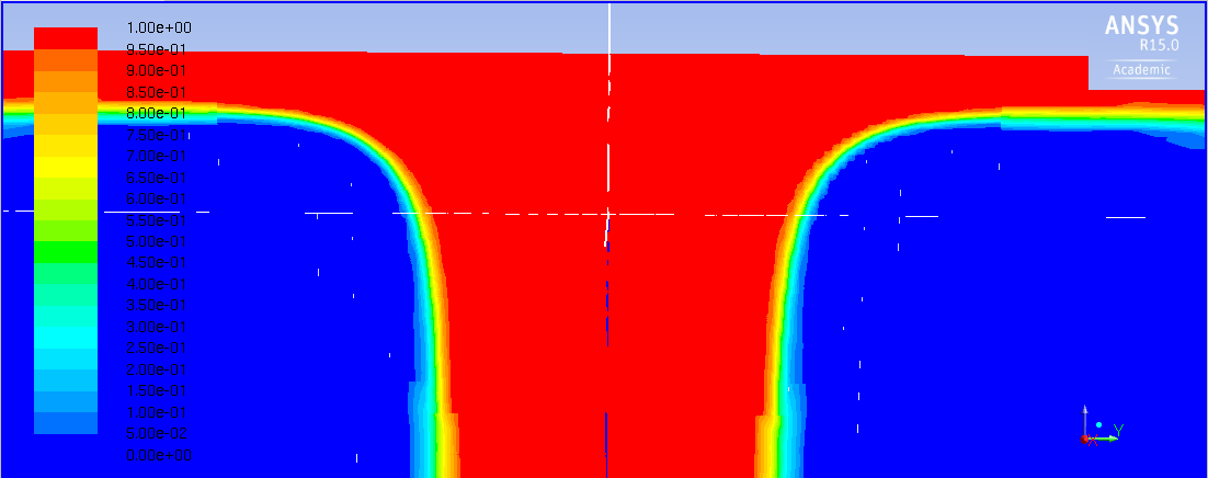
Below are some images of our analysis that we displayed in our presentation.

Below are some images of our analysis that we displayed in our presentation.

 |
| This image is a velocity contour of a vertical plane and the top plate. |
 |
| This is a picture of a calculated impingement area |
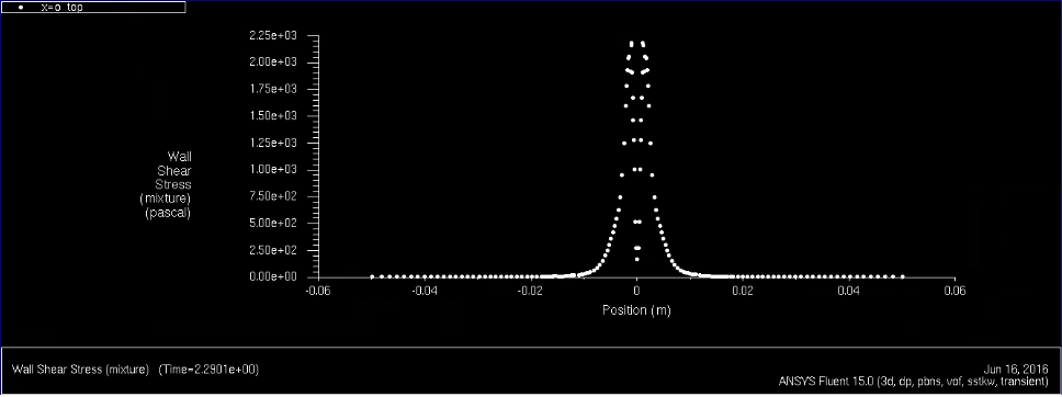 |
| This graph is showing the Wall Shear Stress vs. the vertical position in the cylinder. |
Friday, June 10, 2016
Week Three
The friendly computer folks at OU had an interesting sense of humor when they created the university's servers. After naming the servers after the members of the Beatles, server users now have the choice to use either Paul, Ringo, Harrison or Lennon--each with different computing attributes. Depending on our research needs, we will choose different servers to conduct our simulations. However, when all the servers are down, as was frequently the case this week, we were unable to get very far in generating new data. With the data that we did generate, much of it (on my end, mostly) was determined to be unusable as Fluent autosaved the data as .cdat and .cgns file types, instead of the readable .dat file type. After learning how to prevent this from happening the hard way, we were able to get back on track merely hours before the servers went down (again).
 |
| Picture of the Impingement Area on the bottom of the piston. This was gathered by analyzing the Volume Fraction of Oil in the Cylinder |
For your enjoyment, below are a few pictures of the mesh Morgan worked so tirelessly on. Making a mesh in ANSYS is a lot easier said than done!


Friday, June 3, 2016
Week Two
There has been previous work on oil jet cooling at Oakland University. Graduate student Gary Liu has wrote a complete dissertation on his experimental data of oil jet cooling experiments. Another graduate student, Bolong "Polo" Ma replicated some of Gary's experimental data through CFD simulations. We will be continuing to verify some of these experiments as well as generate new data of our own. This week, we met with Polo to gain a better understanding of his abstract mesh that was used in the simulation. The mesh was highly refined in some areas that needed to be coarsened. In order to adjust these portions of the mesh, a replication of the model needed to be made in the meshing software, ICEM CFD. This new mesh will be used for future simulations However, there were technical issues that hindered our progress in doing so. In order to solve the problem, there needed to be a better understanding of the mesh designer tools, so this week also consisted of working through a few meshing tutorials. The two simulations that needed to be continued began running well. However, there were issues getting the newer simulations running; some of the calculated variables diverged very early. We are still currently looking into solving this issue.
 |
| 1st Oil Jet & Plate Mesh |
 |
| Divergence Error |
Wednesday, June 1, 2016
Week One
Summer 2016 is here and the Automotive and Energy Research Industrial Mentorship Research (AERIM) program at Oakland University is underway! This program, in conjunction with the National Science Foundation is providing aspiring undergraduate engineers with an awesome research and mentorship experience to help develop potential and career interests.
This summer Morgan Jones and myself, Aaron Demers, will be conducting research under Dr. Guessous on an engine cooling project. To preface our research, in today's world the demand for more efficient engines is leading to the development of smaller engines that can produce the same amount or even more power than before. Because of the increase in power density, today's engines are facing somewhat of a cooling problem as increasing thermal loads can cause many issues. Our research is geared towards cooling the bottom of engine pistons using an upward facing oil jet. To achieve this end, we are using ANSYS Fluent 15.0, an advanced Computational Fluid Dynamics simulation software, to simulate and solve for the impingement area of the oil jet on the flat plate of a piston. Optimizing the technology of oil jets is essential to the automotive and energy industry and the usage of CFD programs is becoming an industry standard.
This first week, our group practiced running simulations with ANSYS Fluent using available tutorials online in order to get the hang of using the software. The training included learning how to build geometries, use different CFD solution methods, importing mesh, creating boundary conditions, and analyzing results from the simulation. Understanding the typical workflow for Fluent is imperative for our continuing research. Below are just a few pictures of some of the results we simulated.
 |
| Tutorial 1 : Heat Transfer and Fluid Flow Through a Mixing Tube Elbow |
 |
| Tutorial 3: Heat Transfer and Fluid Flow Through a Heat Exchanger |
 |
| Tutorial 4: Periodic Flow Through a Tube Bank |
Subscribe to:
Posts (Atom)