Week Five

This week Morgan and I were back at it inside our simulation cave. We achieved some good progress in analyzing the 7.35 and 3.64 m/s cases. Instead of first telling you about it, I'll show you some interesting pictures we generated in CFD-Post and then describe them to you.

What these cool jellyfish-like pictures are showing are the streamlines of the oil at the impingement area. We can see how and where the downward streams are developing. One thing we would like to do is investigate why they are developing in a given area as well as why they are not equidistant from each other, given an equal surface tension parameter.

Here we have a bottom view where we can see the streamlines forming off of the impingement area. At the very bottom, we have a gathering cluster of streamlines. While most of these will inevitably find their way to the stream to the left and right, we have seen that this is where some drops of oil have fallen. With a slight increase in velocity, we believe this could be where the 6th stream is supposed to develop.

In this picture we have a side view of a section of the impingement area. We can easily estimate the thickness, however, we would like to quantify the thickness of the impingement area as a function of the radial velocity and velocity gradient.

Week Four

This was indeed a very packed and exciting week filled with analysis, meetings, presentations, and vehicle test-driving. Monday and Tuesday were spent doing data analysis on the 7.35 and 3.64 m/s cases. Additionally, we were preparing for our presentation on Wednesday. After said presentation on Wednesday, Morgan and I met with Dr. Guessous and Sangeorzan to discuss the results of our project as well as its future direction. We want to be able to characterize the thickness of the impingement area and relate it to the radial velocity gradient with respect to increasing height (as the stream gets closer to the plate). For the 3.64 m/s inlet velocity case, we calculated the mass and volume flow rates of the streams coming down and compared it to that of Gary Liu's experimental data with great accuracy. In the process of this calculation we found the average velocities and area of the streams as a total amount. Next week, one of the things we will be doing is looking at the individual area and velocities of each stream at givens points.

As I briefly mentioned earlier, there was a lot of out-of-lab activities going on. We had a presentation given by Dr. David Wagner on light weight vehicle materials. He gave us the lowdown of material properties in vehicle structures and what goes into making decisions about what materials will comprise a new model vehicle. On Friday we went to Chrysler's wind tunnel. This was an awesome experience in which we got to see how engineers in industry do aerodynamic testing on their vehicles. Furthermore, we were able to explore Chrysler's state-of-the-art wind tunnel circuit and learn about the subtleties involved in making a good wind tunnel. To cap off the week, we went to the Young Automotive Professionals Conference at GM's Proving Grounds. In the morning we had the privilege of hearing from the industry's leading developers automotive world. It was quite interesting to see how technology is and will drastically shape the world we live in. From automated driving to vehicle cyber security to vehicle ride-sharing, it was all intriguing material. For example, one of the things they talked about was a newly developed program called Maven, an urban ride-sharing smart phone app that would allow people to seamlessly rent a vehicle from a lot for a couple of hours, or even a weekend. This would drastically reduce city parking lot congestion as well as parking permits, which in many cities can be up to $400-500 a month.

Below are some images of our analysis that we displayed in our presentation.

This image is a velocity contour of a vertical plane and the top plate.

This is a picture of a calculated impingement area

This graph is showing the Wall Shear Stress vs. the vertical position in the cylinder.

Week Three

The friendly computer folks at OU had an interesting sense of humor when they created the university's servers. After naming the servers after the members of the Beatles, server users now have the choice to use either Paul, Ringo, Harrison or Lennon--each with different computing attributes. Depending on our research needs, we will choose different servers to conduct our simulations. However, when all the servers are down, as was frequently the case this week, we were unable to get very far in generating new data. With the data that we did generate, much of it (on my end, mostly) was determined to be unusable as Fluent autosaved the data as .cdat and .cgns file types, instead of the readable .dat file type. After learning how to prevent this from happening the hard way, we were able to get back on track merely hours before the servers went down (again).

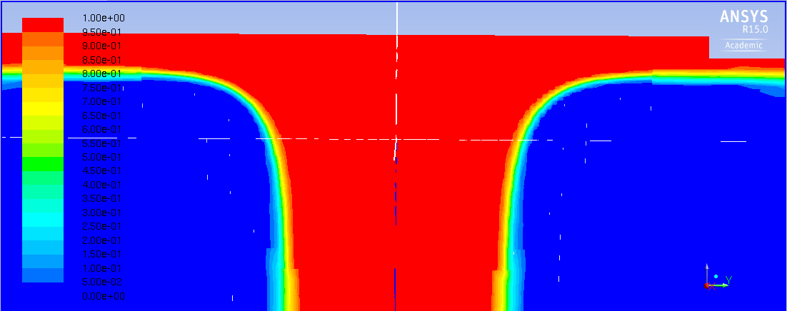
Besides data and server issues, we did happen to make some good progress. For one, after copious amounts of meticulous work, we were able to generate a pretty good mesh that will be used for our next set of simulations. For these simulations, we are modeling the piston to be at mid-stroke (further away from the jet nozzle), instead of at the bottom of its stroke where our current simulations are taking place. Additionally, we calculated the jet impingement areas for the 3.64 and 7.35 m/s 60°C cases. We did this using a feature called Iso-Clip, which we used to cut out the area in which there wasn't any oil present (the blue area in the picture below) and subtracted that from the total area of the piston in order to obtain the effective impingement area (the red area with a greenish border). We then compared this calculation to the experimental data generated by Gary Liu, a PhD student worked on this project in years past.

Picture of the Impingement Area on the bottom of the piston. This was gathered by analyzing the Volume Fraction of Oil in the Cylinder

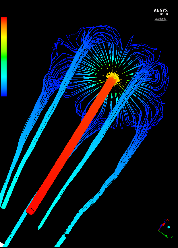
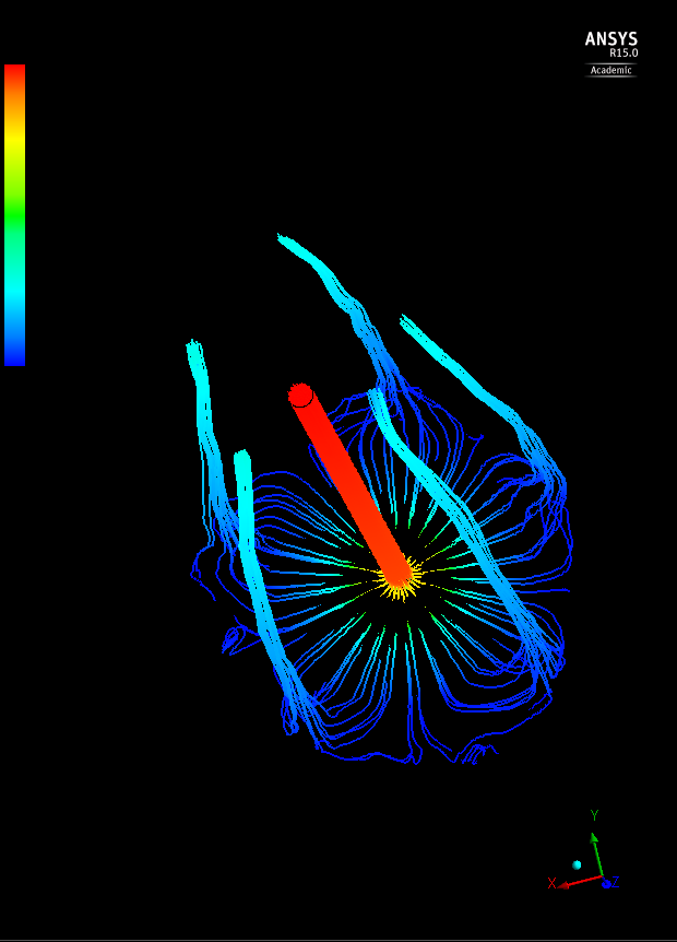
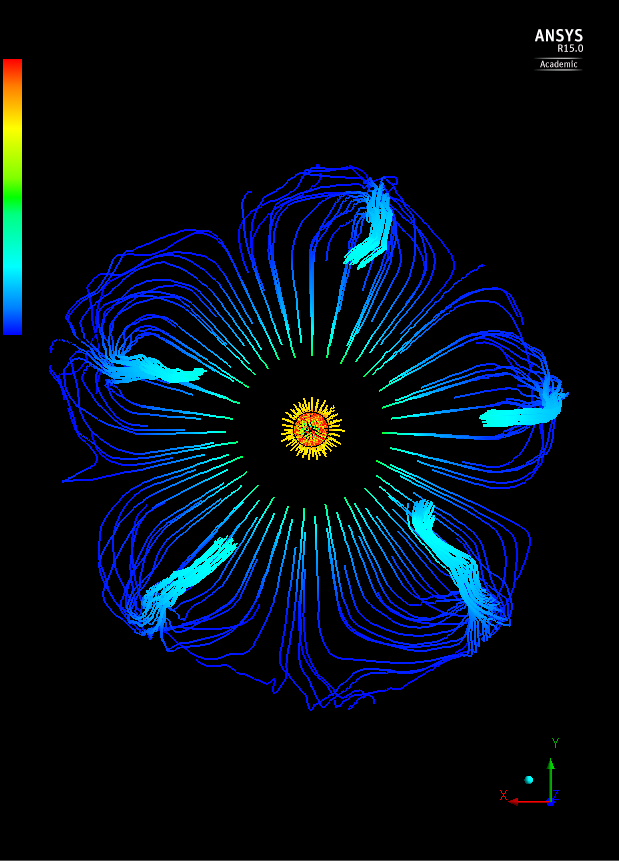
For your enjoyment, below are a few pictures of the mesh Morgan worked so tirelessly on. Making a mesh in ANSYS is a lot easier said than done!

Week Two

There has been previous work on oil jet cooling at Oakland University. Graduate student Gary Liu has wrote a complete dissertation on his experimental data of oil jet cooling experiments. Another graduate student, Bolong "Polo" Ma replicated some of Gary's experimental data through CFD simulations. We will be continuing to verify some of these experiments as well as generate new data of our own. This week, we met with Polo to gain a better understanding of his abstract mesh that was used in the simulation. The mesh was highly refined in some areas that needed to be coarsened. In order to adjust these portions of the mesh, a replication of the model needed to be made in the meshing software, ICEM CFD. This new mesh will be used for future simulations However, there were technical issues that hindered our progress in doing so. In order to solve the problem, there needed to be a better understanding of the mesh designer tools, so this week also consisted of working through a few meshing tutorials. The two simulations that needed to be continued began running well. However, there were issues getting the newer simulations running; some of the calculated variables diverged very early. We are still currently looking into solving this issue.

1st Oil Jet & Plate Mesh

Divergence Error

Week One

        Summer 2016 is here and the Automotive and Energy Research Industrial Mentorship Research (AERIM) program at Oakland University is underway! This program, in conjunction with the National Science Foundation is providing aspiring undergraduate engineers with an awesome research and mentorship experience to help develop potential and career interests.

This summer Morgan Jones and myself, Aaron Demers, will be conducting research under Dr. Guessous on an engine cooling project. To preface our research, in today's world the demand for more efficient engines is leading to the development of smaller engines that can produce the same amount or even more power than before. Because of the increase in power density, today's engines are facing somewhat of a cooling problem as increasing thermal loads can cause many issues. Our research is geared towards cooling the bottom of engine pistons using an upward facing oil jet. To achieve this end, we are using ANSYS Fluent 15.0, an advanced Computational Fluid Dynamics simulation software, to simulate and solve for the impingement area of the oil jet on the flat plate of a piston. Optimizing the technology of oil jets is essential to the automotive and energy industry and the usage of CFD programs is becoming an industry standard. 

This first week, our group practiced running simulations with ANSYS Fluent using available tutorials online in order to get the hang of using the software. The training included learning how to build geometries, use different CFD solution methods, importing mesh, creating boundary conditions, and analyzing results from the simulation. Understanding the typical workflow for Fluent is imperative for our continuing research. Below are just a few pictures of some of the results we simulated.

Tutorial 1 : Heat Transfer and Fluid Flow Through a Mixing Tube Elbow

Tutorial 3: Heat Transfer and Fluid Flow Through a Heat Exchanger

Tutorial 4:  Periodic Flow Through a Tube Bank