Week Eight

With our time at Oakland University starting to wind down, Morgan and I spent a great deal of time this week organizing data in order to implement it in our paper and poster presentation. Along with this work we attended an interesting lecture on internal combustion engines given by Dr. Zhao, a new professor at Oakland University who graduated from Princeton. Additionally, we attended a poster presentation workshop given by Dr. Dean, where he covered the Do's and Don'ts and other guidelines for giving an effective poster research presentation. This workshop came at a great time, as the MID-SURE Undergraduate Research Conference is being held at Michigan State University on July 27, less than 2 weeks away!

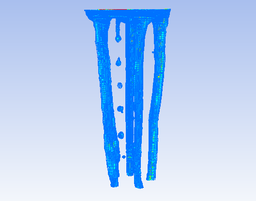
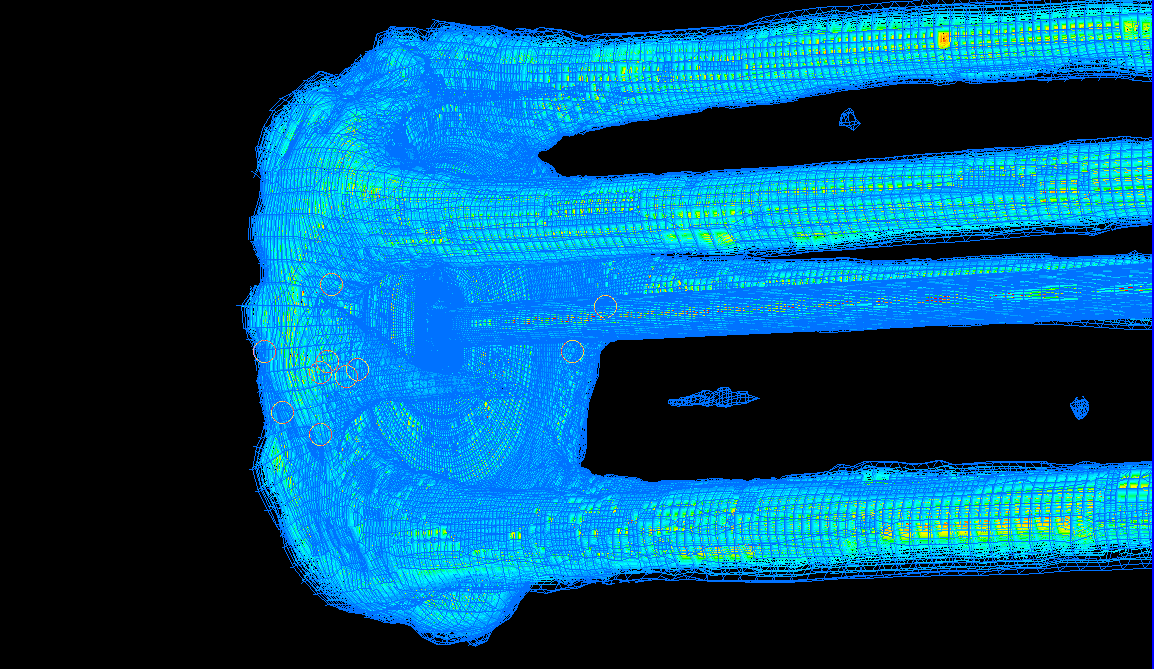
With all that being said, there was still plenty of research going on in our little Dodge Hall enclave. We generated some good plots that illustrates and compares the hydraulic jumps of our three cases. Below is some delicious eye candy, courtesy of Morgan Jones.

Here we are looking at the edge of the impingement area in a region between two streams. This bubble-like formation is a hydraulic jump. Also, notice how the distance progressively gets larger and larger away from the origin. This is just showing that given a higher flow rate, the impingement area is bigger.

Intermission time. Whilst perusing the Internets for a CFD question we were interested in, I found a thread on a CFD help forum with a few CFD-related jokes, if you could imagine there would be such a thing! A few sardonic individuals came up with some quippy mnemonics for CFD that I thought I would share with you:

CFD - Colorful Figure Delivery

CFD - Colors for Directors

CFD - Cleverly Forged Data

You can't deny that there isn't at least a small bit of truth to these...

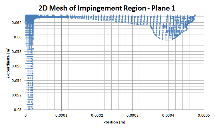
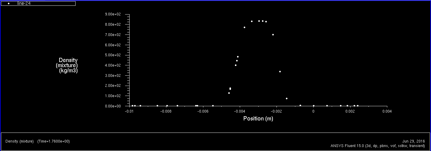
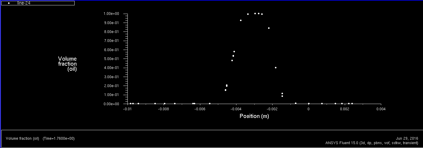
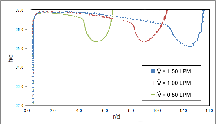
Back to business! As we defined at the beginning of the summer research, one of the most important things we wanted to look at was the impingement area for the three cases. That is, given a certain flow rate, how big is the impingement area going to be and how much is that going to cool down the piston? Below is a graph comparing the impingement areas for our three cases:

Quantitatively speaking, the 1.0 LPM case's impingement area is 57% larger than the 0.5 LPM case. Furthermore, the 1.5 LPM case area is 69.8% and 166.5% larger than the 1.0 and 0.5 LPM cases, respectively. In short, if you squirt more oil at the bottom of the bottom of the piston, the more the piston will get cooled down. However, it's not that simple as there are other important parameters to look at; such as possible oil misting and parasitic engines losses from the oil pump. Further research is being done (though not currently by us) on how much oil is ideal for cooling down pistons.

Well, folks, that's it for this week. Be sure to come back next week for more exciting CFD news from Dodge Hall!

Week Seven

After a relaxing 4th of July weekend, Morgan and I were back in the lab doing data analysis and working on the American Society of Thermal and Fluids Engineers (ASTFE) paper. Although the paper isn't due until September, we've been chipping away at it to make things considerably easier in the future. The big motivation behind writing this paper is to get it published and to attend the ASTFE conference in Las Vegas next April where we'll present our project. 

As the weeks go by, we've been making steady progress with both the paper and the data analysis. After some grid-mesh adaptions we made last week the simulations powered through the weekend to yield some interesting results for us this week. For the 11 m/s case, we refined the grid near a section where two streams were merging together. After letting that case run for a few more days, we found that the streams had separated. Whether that's due to our mesh adaption or a yet-to-be-discovered flow pattern, it is not clear. 

This week we also calculated the distances between the streams for the three cases, as well as the average distance. It seems that the average distance for all the cases is between 1.32 and 1.37 cm, regardless of how many streams the case may have. In addition, we calculated the impingement area for each case as a function of time, but focusing on the small fluctuations that are observed at near-steady state. We can't say that any given case reaches exactly steady state as there are always slight changes in the area, but for all intents and purposes, these changes are so small that any deviation from the average value is negligible.  

As a highlight, this week Morgan found a new way to calculate the jet impingement region thickness. The old way involved manually converting polar coordinates to Cartesian coordinates to generate a given plane. Once that plane was made, lines were created at set distances within those planes with their values plotted in order to get a select few thickness values. These lines and planes were meticulously created between and at stream locations. As thrilling as that sounds, Morgan decided to reinvent the wheel of tedious plane analysis. However, he not only reinvented the wheel, he created a Mercedes Benz Silver Lightning method of finding these thickness values. Behold! Feast your eyes upon the glory of Morgan's Method:

This is so much more than your ordinary, every day Microsoft Excel plot. What you are seeing is a revolutionary way of doing CFD analysis. Simply scroll your mouse over a point, and it will give you a representative thickness value! (Hint: you can't actually scroll over this image to get a value, you'll have to come to our lab to have access to our Top Secret Excel documents.)

Like any good invention, the highly-coveted secrets behind this method are patented (pending) and are reserved only for the most privileged members of the Oakland's prestigious CFD community...

Week Six

Welcome back! This week there weren't any AERIM events to go to so we had plenty of time to use towards lab work and meeting with Dr. Guessous and Sangeorzan to discuss our results. During these meetings, we found that it was necessary to do a little digging in order to find the best Volume Fraction (VF) cut off range for our data analysis. This volume fraction cut off point is used to show the area of oil on a given plane. If it is too low, as in the picture below, our area will include too much air. If it is too high, one may be neglecting too much oil and thus the mass flow rate is drastically reduced.

This is an oil Volume fraction from 0 to 1. Notice that this is the area
 of the entire top plate because it also includes air in its area calculation.

This is an impingement area where the Volume Fraction cut off is a 0.05, or 5%.

So, in order to effectively consider our VF cut off point, we made plots of density and Volume Fraction at certain distances across the cross-section of a stream. The way Fluent calculates Mass Flow Rate is based off of density. Additionally, there is a direct correlation between density and the volume fraction cut off, as can be seen below.

After doing much more analysis concerning the VF cut off point, we decided that a cut off point of 5% would be optimal as it not only clips out the air from calculations, but it also contains the bulk of the oil.

In other news, we're also investigating the formation of a stream on our 3.64m/s case.  Below is an image of a drip that is not quite a stream yet. We're refining the mesh here and continuing this simulation to see if indeed a full-fledged stream forms.

A prettier, side angle view that shows the early formation of a stream.